Lab 7 - Kalman Filter

Estimate drag and momentum

The picture provided below is the screenshot from the lecture notes. We have to find the steady-state velocity and the 90% of the rise time. Based on the data collected from step response, I generated the plots for the ToF, PWM, and velocity vs. time.

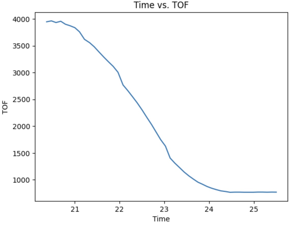
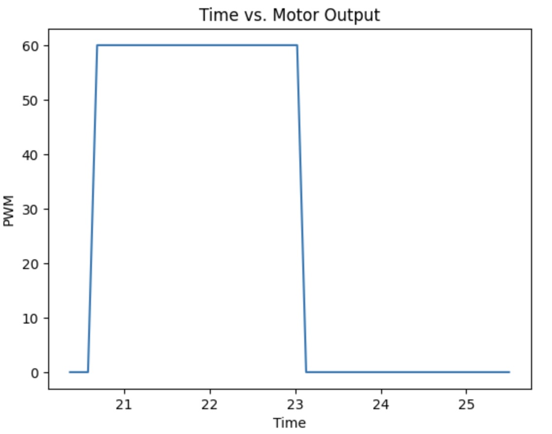
All the plot needed is provided above. The PWM I choose is 60, which is average of the motoroutput I get form lab 6. The car start moving 4m far from the wall to make sure it can reache the steady state velocity. From the plot, the steady-state velocity is 2100mm/s. The velocity plot is not perfect, but due to the low on time, I still choose to use this set of data. We could still realize the robot reaches the steady-state velocity and it lasts for a while. The 90% of the rise time can also get directly from the plot, which is around 1.5s.

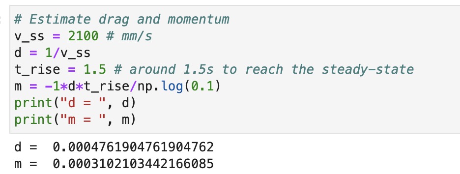
Based on the lecture notes provided, d = u/(steady-state velocity) and m = -d*(90% of the rise time)/ln(0.1). Note, we assume u = 1 for now. The picture above shows the calculation process in Python to get the drag and momentum.

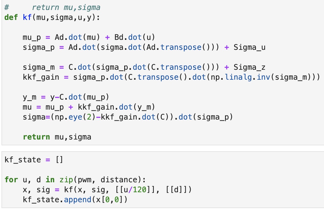
Initialize KF

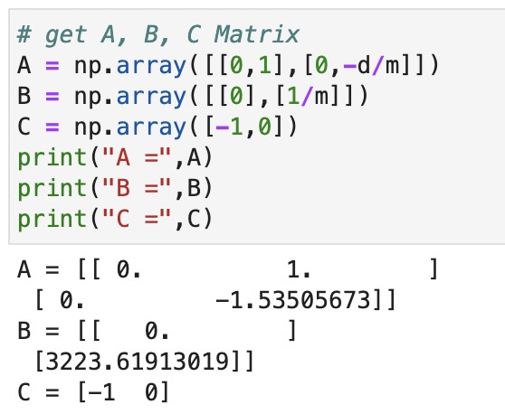
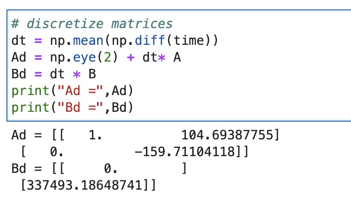
Based on the term I found above, the state-space equation can be calculated by using the lecture notes provided at the very top. And then I discretize the matrices. The sampling time I use is the average sampling time from the step response.

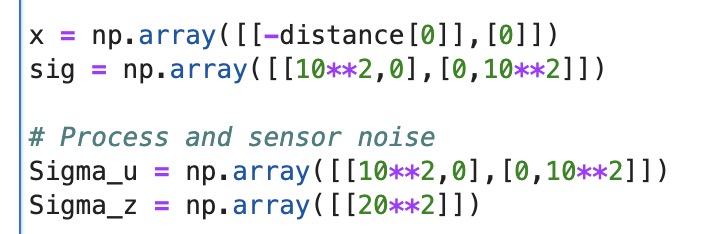
The last step of the initialize the Kalman Filter are to initialize the state vector and specify process noise and sensor noise covariance matrices. Sigma 1 and 2 are set to be 10 for now and it will do some further adjustment in the next section. Sigma 3 is set to be 20 based on the lecture provided.

Implement and test your Kalman Filter in Jupyter

By implementing the code example provided in the lab instruction for the Kalman Estimation, I can then run it to get the estimation data. I rerun the lab 6 code to get a new set of data to do the sanity check.

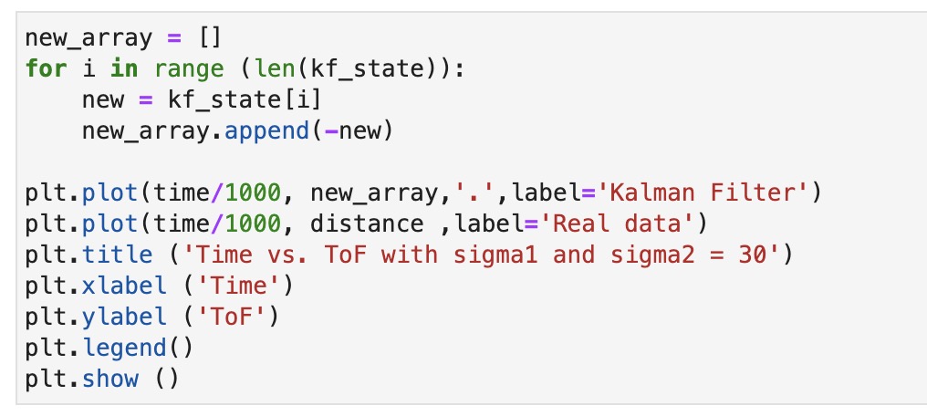
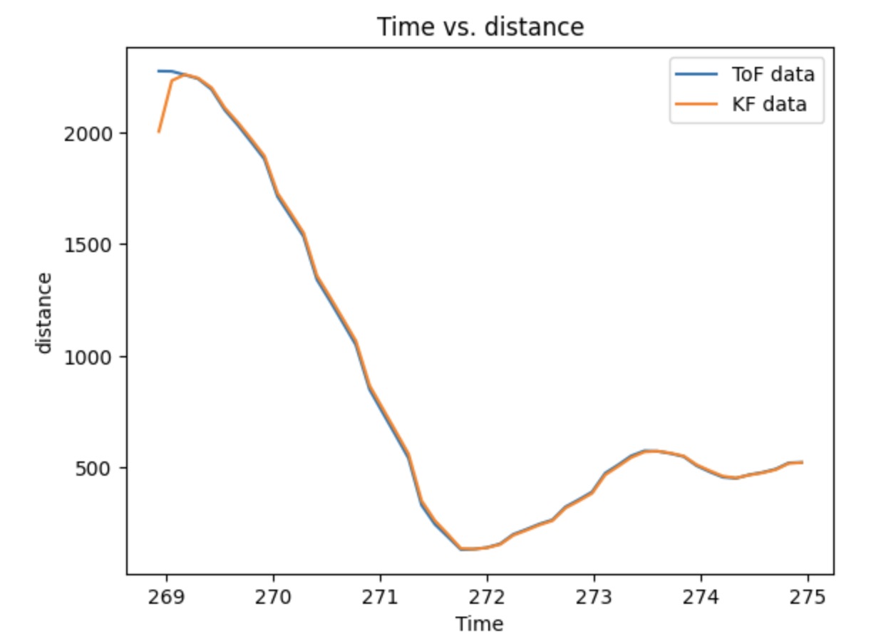
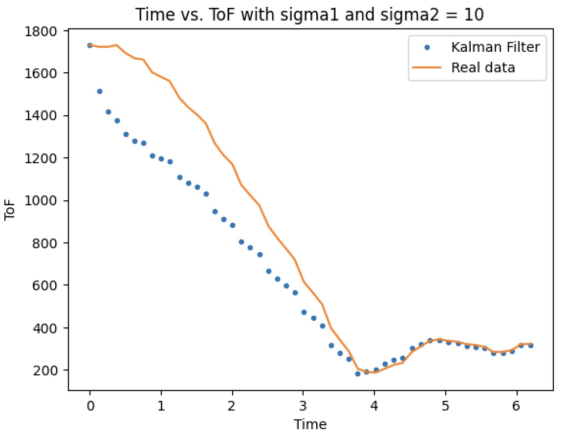
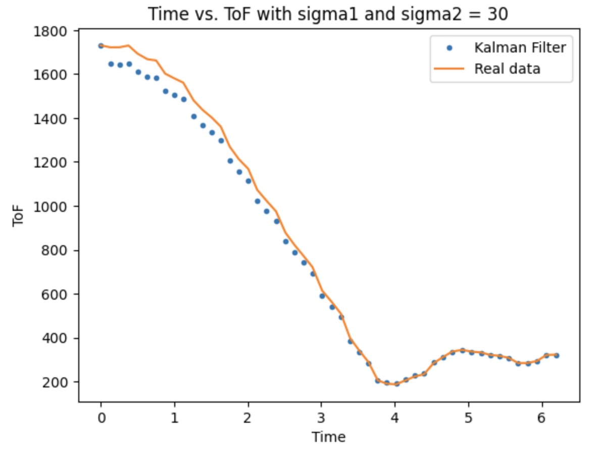
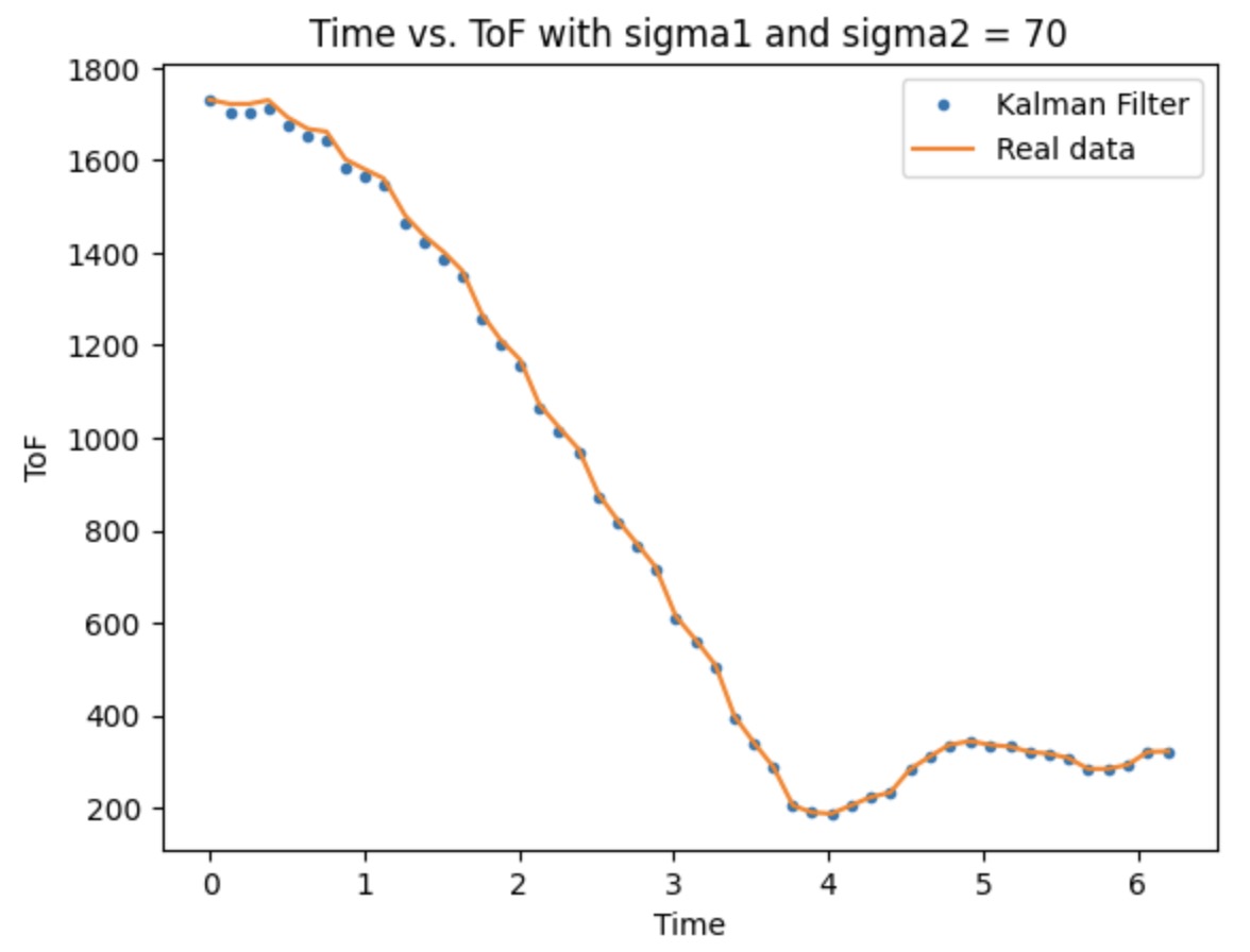
The picture provided below shows the sigma 1 and 2 adjustment process. The default value I set before is 10, which is not reach to what we expected. Therefore, I tried to increase the value until 70. The Kalman Filter can almost perfect fit the real data.

Extrapolation

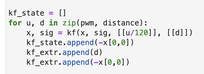
When doing the extrapolation, we want to estimate the distance value between the sampling interval to make our robot to react faster. So, first, we have to set the extrapolation time interval to be smaller than sampling interval. I set it to be half than before here. Then, arrange the time array and get the extrapolated data, which is similar as the task above.

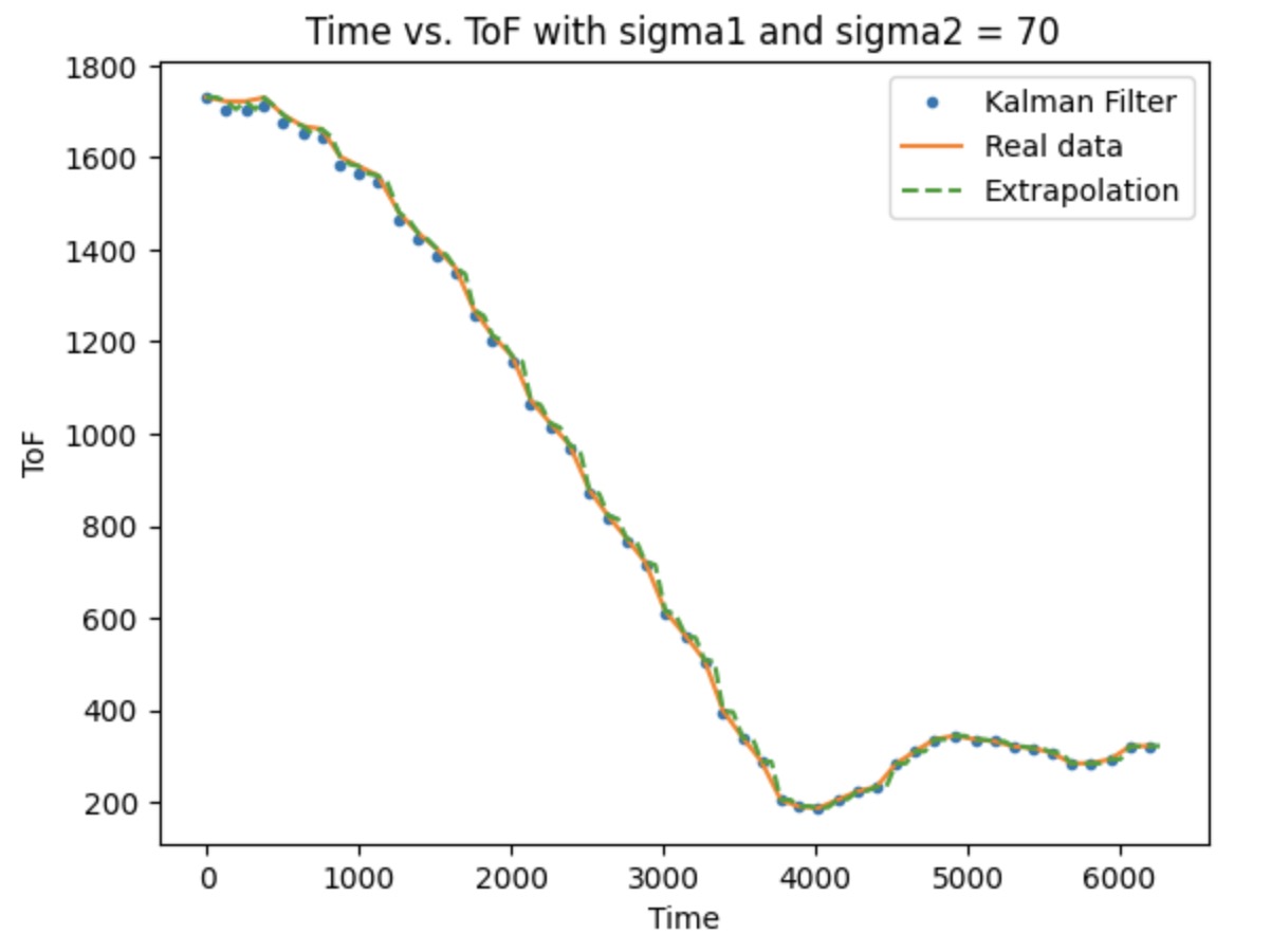
The plot including the extrapolation is shown below.

KF Implementation

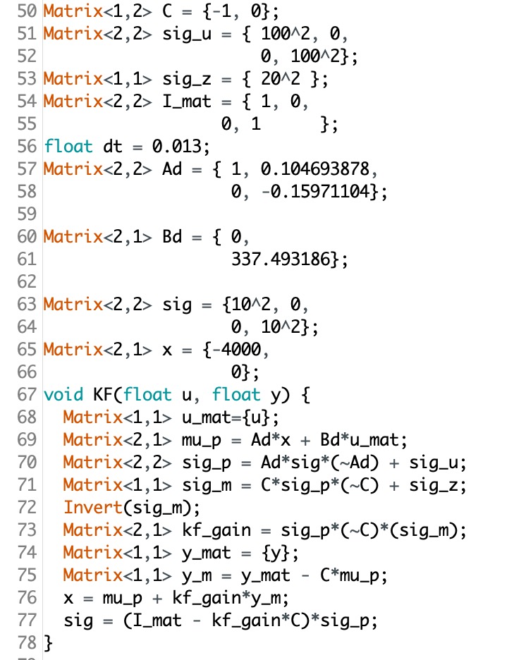
The code below shows the KF implementation process by converting the Python code into the Arduino type code.

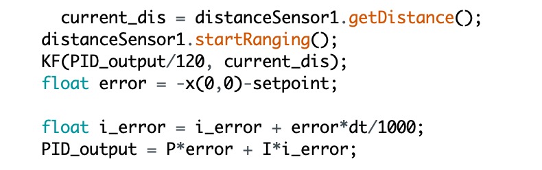
This code shown below represents how the new error would be to calculate the PID output(pwm).

The video below shows the KF works well when it applies to the real robot. It do increase the speed a little bit compared with the one I did in lab 6.