Lab 9 - Mapping

Control

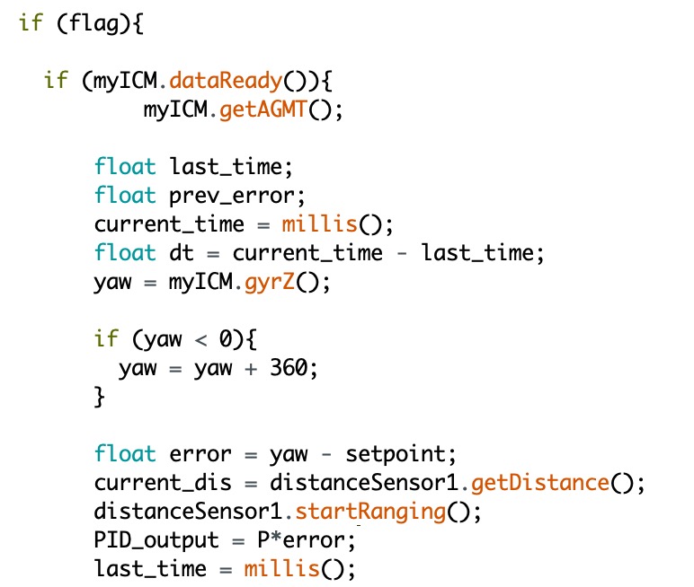
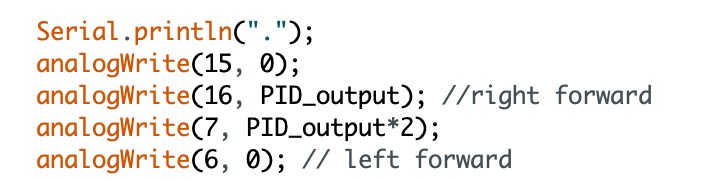
In this lab, we are required to do the PID controlling for the IMU to get the surrounding map by turning the robot on-axis. I choose to achieve this using Angular speed control. The data collection is easier than doing the orientation control. We can just get the angular speed by using the yaw value provided by the IMU. We just care about the rotation that is parallel to the floor, so yaw itself is good enough in this lab. In this case, the error in the PID calculation should be the yaw value minus the setpoint. I set it to be 15 to try to lower the rotational speed and controller will make sure our robot can rotate around the speed of 15 deg/ms Then I apply the PID function to get the output and I only use P control here. The last step is to set the PWM value, which equals to the PID output value. My code is attached below.

The video below shows my robot can successfully rotate at a relatively slow angular speed with just a small drift. It is driving in a straight circle, not on-axis. At very beginning, when I run my code, the left side of the wheel seems to stop. I try both stick the tape on the wheels and do the PWM calibration, but both them are not working very well. The final version still contains the drift, but I don't think it will cause too much error, which is acceptable.

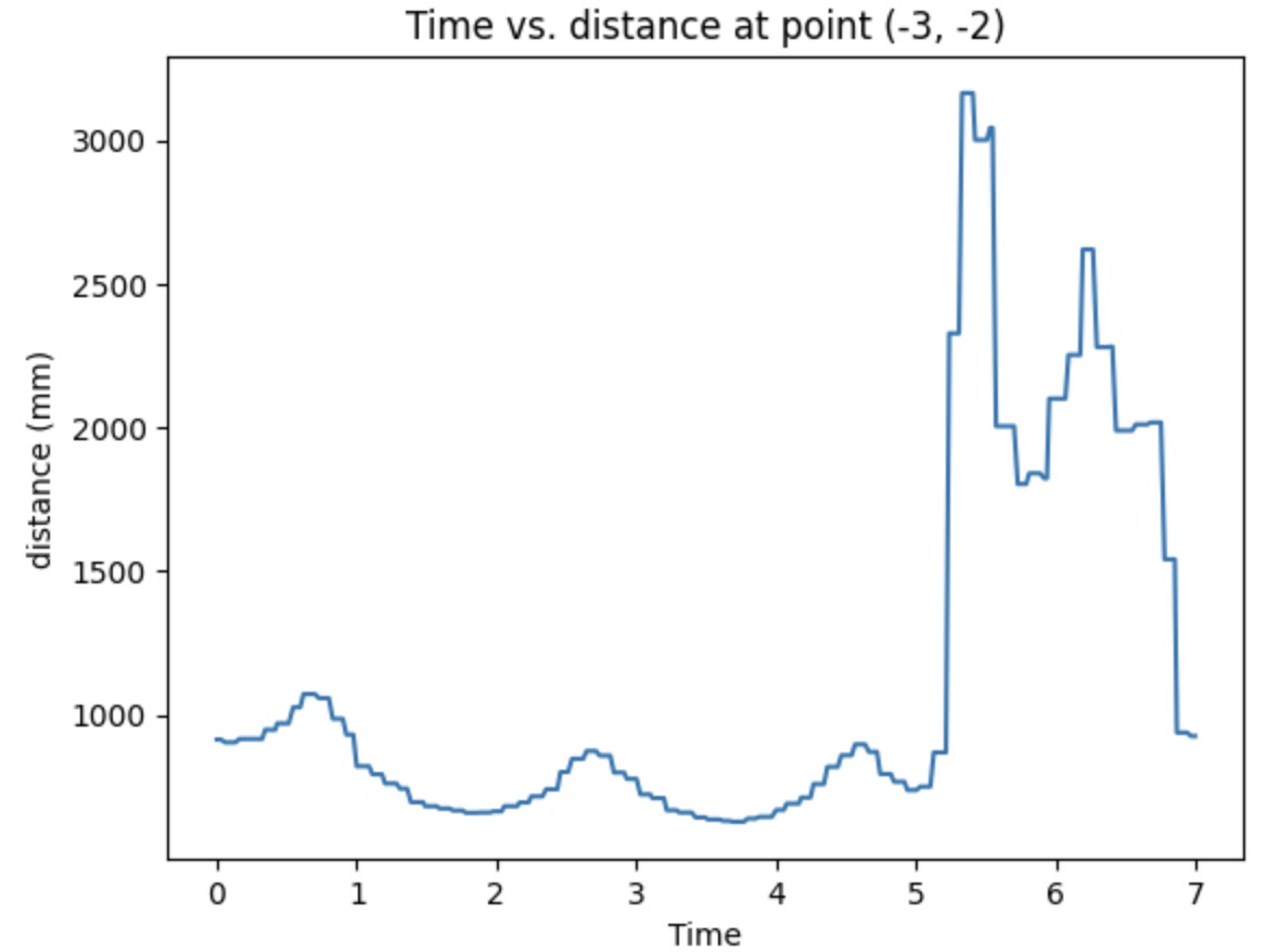
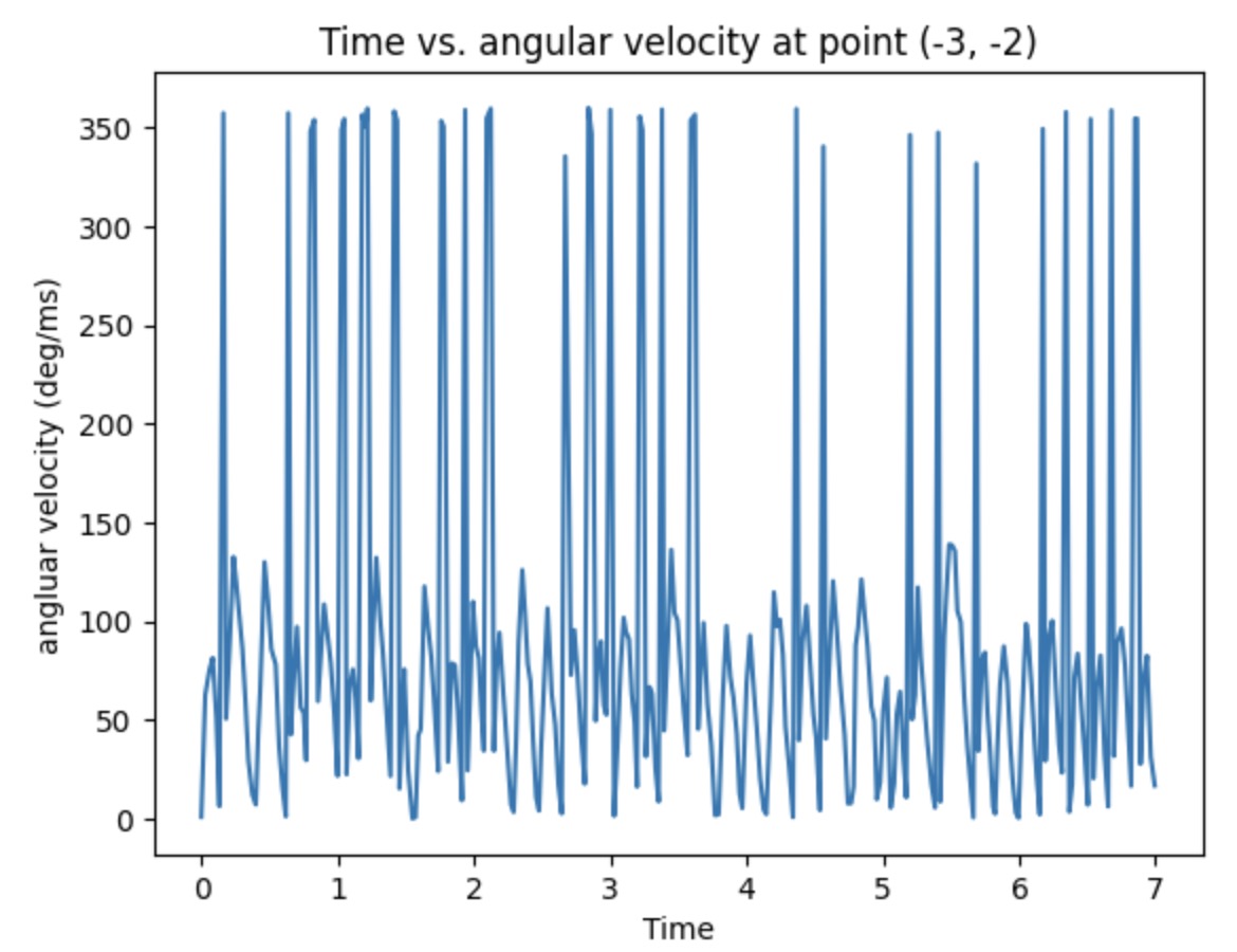
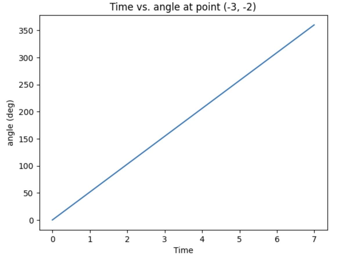
The plots below show the time vs. IMU data, ToF data, and the angle value I calculated by using the angular speed times the time difference. The plotted data is gathered from the testing point (-3,-2) in first run. The distance plot is reasonable with some suddenly increased and decreased value. For the angular velocity plot, I think I might mess up the unit. However, it seems that the rotational speed can be controlled at a constant value. Then I calculate the sum of the angle andn the plot looks perfect with the range from 0 to 360.

Read out Distances

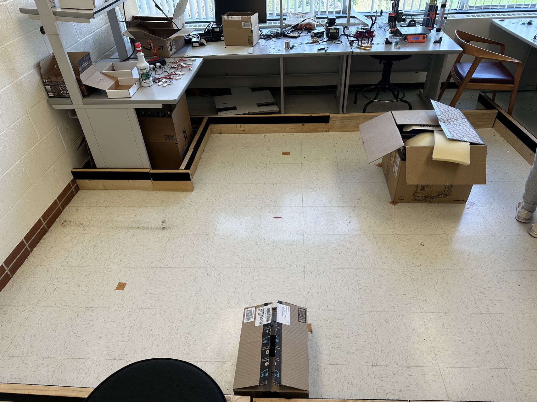
The picture below is the real map set up to use in this lab. There are five marked position on the floor, which labeled as (-3,-2), (5,-3), (0,3), (0,0),(5,3). We could use the robot to record the distance at these five points separtely.

The pictures shown below are the polar plot for each testing point. I did 2 runs in total and gathered them into the same plot. It clear that it is more accurate when measuring the object with short distanc and with the distance increased, the accuracy will decrease. As you can see on the plot, the shorter distance recorded for the run 1 and run 2 are almost overlaped, which means the data is exactly what I expected.

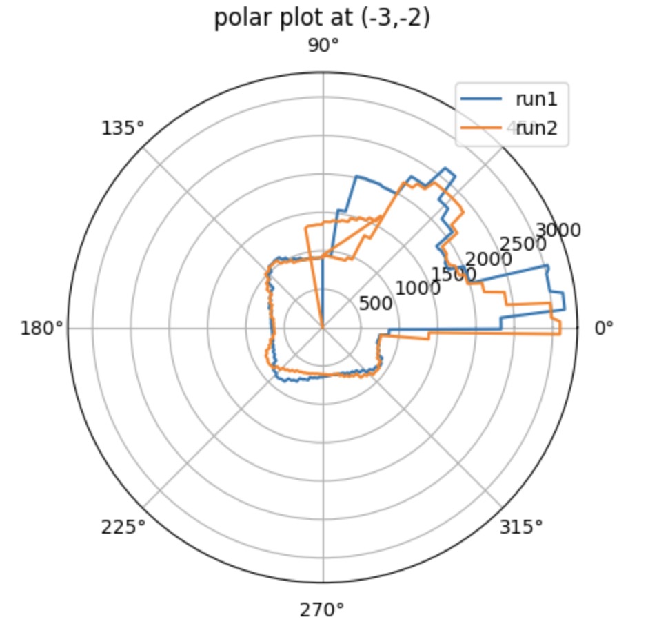
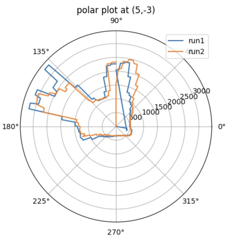
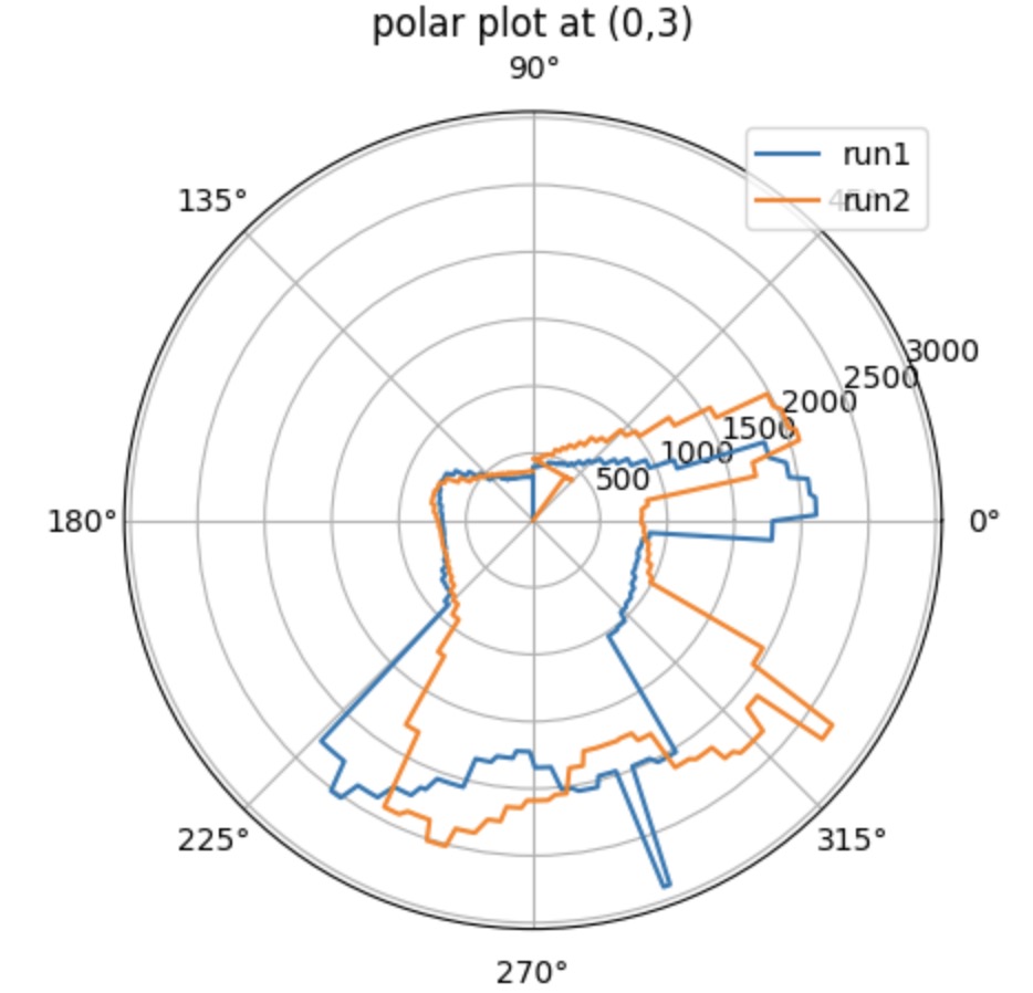
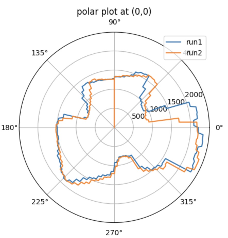
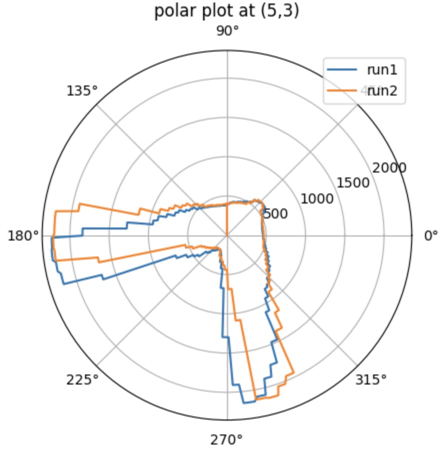
When recording the data, the sensor should start with the same orientation at each coordinate. To match the direction for the obstacles orientation shown in the real map, I rotate my data 90 degrees counterclockwise.

Merge and Plot your readings

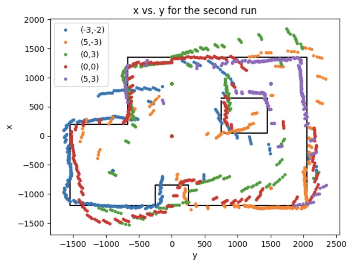
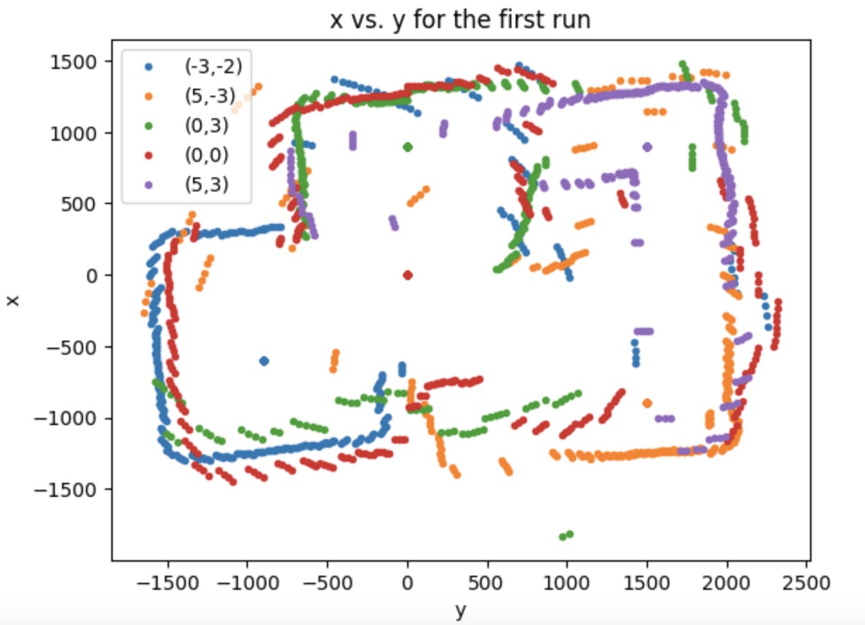
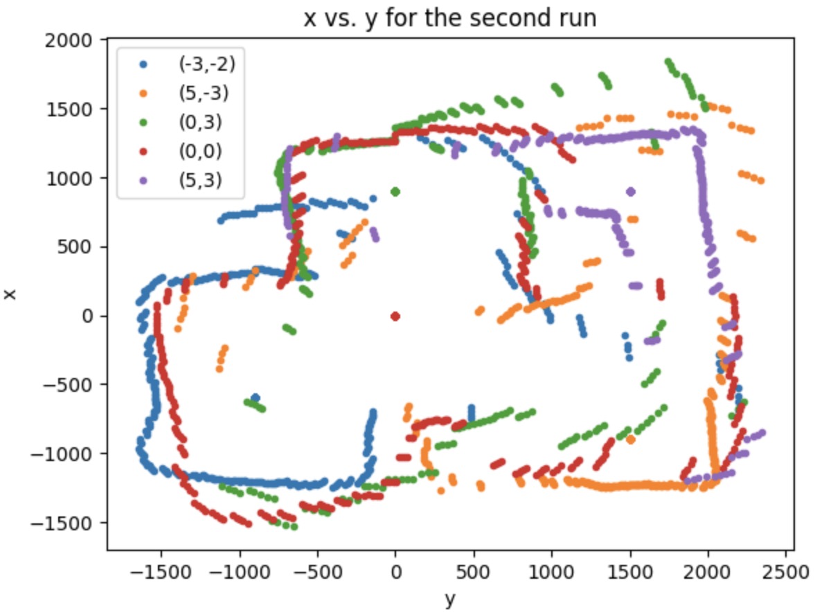
Then, to finally get the plot shown like a real map, we should convert our plot from polar coordinate into Cartesian coordinate. I use the equation: x = distance * cos(theta) and y = distance * sin(theta) to get the x and y value. According to the material provided in Lecture 2 about the transformation matrics, I can relocate each set of data to the right position. Because I start at the same orientation when doing the testing, there's no rotation happened. What I have to do is to deal with the translation. The point (0,0) is at the origin. Therefore, we need to do the translation manipulate for the rest of the points. The unit of the points coordinates are in feet, so I transfer them into mm by multiplying 300. The map for the 2 runs are shown below, which is pretty similar.

Convert to Line-Based Map

To convert the map into a format we can use in the simulator, I manually estimate where the actual walls and obstacles. To do that, I estimate the coordinate of each turning corner and continuously refine for it by using the map for the run 1. The points are listed below.

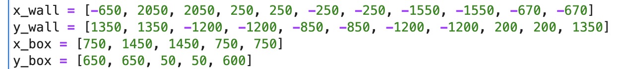
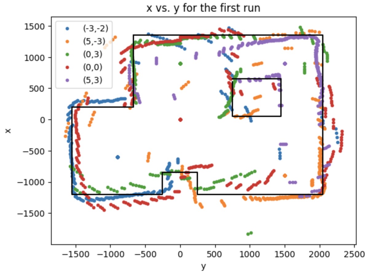
Then I apply the same line_based map onto the run2, it also fit perfectly.